import pandas as pd
import numpy as np
import matplotlib.pyplot as plt
import pandas_datareader as pdr
import datetime as dt
import statsmodels.formula.api as smf
import statsmodels.api as sm

from statsmodels.tsa.filters.hp_filter import hpfilter
from statsmodels.graphics.tsaplots import plot_acf
This section aims to introduce the most fundamental skills of wrangling time series data in Python, specifically with Pandas.
Why Taking Logs?
If the time series that exhibit any traces of growth or decline, i.e. nonstationary, a useful transformation is to take natural logarithm of it. Suppose if \(y_t\) is an observation of the time series in period \(t\), the growth rate from period \(t-1\) is \[ g_t = \frac{y_t}{y_{t-1}}-1 \] where \(g_t\) is the growth rate. Rearrange and take natural log \[ \ln{(1+g_t)}=\ln{\bigg(\frac{y_t}{y_{t-1}}\bigg)}=\ln{y_t}-\ln{y_{t-1}} \] So the question is what is \(\ln{(1+g_t)}\)?
In calculus class, we have learned Taylor Expansion, which is the ultimate weapon for approximate any functions. \[ \ln (1+x)=x-\frac{1}{2} x^{2}+\frac{1}{3} x^{3}-\frac{1}{4} x^{4}+\ldots=\sum_{k=1}^\infty(-1)^{k+1}\frac{x^k}{k} \]
Because the growth rate is usually small, we can use the linear term exclusively in Taylor expansion \[ \ln{(1+x)}\approx x \] which means log difference approximates the growth rate \[ \ln{y_t}-\ln{y_{t-1}} \approx g_t \]
Let’s take a look at real GDP per capita from US.
start = dt.datetime(1950, 1, 1)
end = dt.datetime(2021, 10, 1)
df = pdr.data.DataReader(["A939RX0Q048SBEA"], "fred", start, end)
df.columns = ["R_GDP_PerCap"]
df["R_GDP_PerCap_tm1"] = df["R_GDP_PerCap"].shift(1)
df = df.dropna()
df.head()| R_GDP_PerCap | R_GDP_PerCap_tm1 | |
|---|---|---|
| DATE | ||
| 1950-04-01 | 15977.0 | 15559.0 |
| 1950-07-01 | 16524.0 | 15977.0 |
| 1950-10-01 | 16764.0 | 16524.0 |
| 1951-01-01 | 16922.0 | 16764.0 |
| 1951-04-01 | 17147.0 | 16922.0 |
fig, ax = plt.subplots(figsize=(12, 8))
ax.plot(np.log(df["R_GDP_PerCap"]))
plt.show()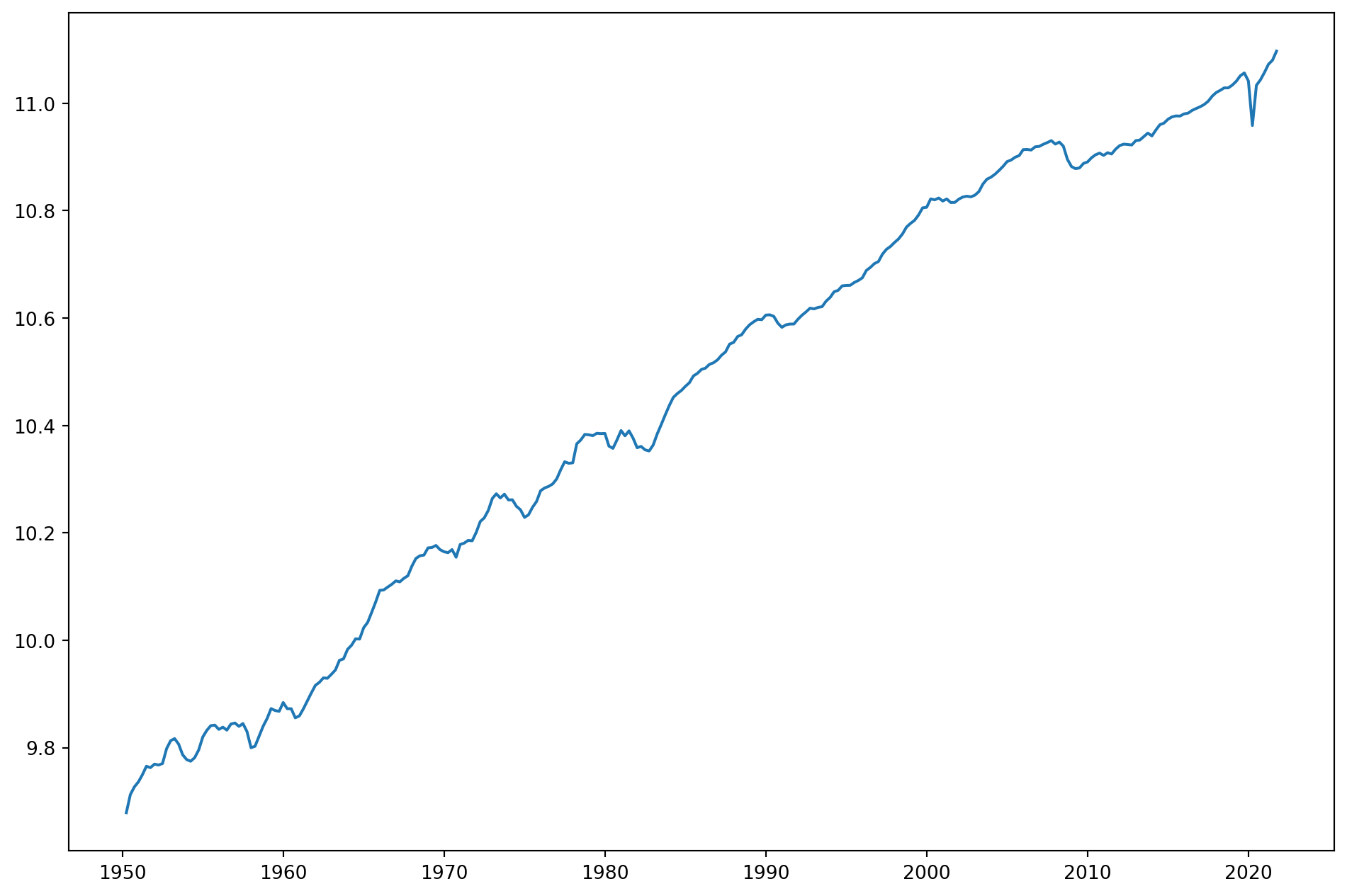
pd.options.mode.chained_assignment = None  # without this, there will be error msg 'A value is trying to be set on a copy of a slice from a DataFrame.'
df["Gr_rate"] = df["R_GDP_PerCap"] / df["R_GDP_PerCap_tm1"]
df["Gr_rate"] = df["Gr_rate"] - 1
df.head()| R_GDP_PerCap | R_GDP_PerCap_tm1 | Gr_rate | |
|---|---|---|---|
| DATE | |||
| 1950-04-01 | 15977.0 | 15559.0 | 0.026865 |
| 1950-07-01 | 16524.0 | 15977.0 | 0.034237 |
| 1950-10-01 | 16764.0 | 16524.0 | 0.014524 |
| 1951-01-01 | 16922.0 | 16764.0 | 0.009425 |
| 1951-04-01 | 17147.0 | 16922.0 | 0.013296 |
df["Gr_rate_log_approx"] = np.log(df["R_GDP_PerCap"]) - np.log(df["R_GDP_PerCap_tm1"])
df.head()| R_GDP_PerCap | R_GDP_PerCap_tm1 | Gr_rate | Gr_rate_log_approx | |
|---|---|---|---|---|
| DATE | ||||
| 1950-04-01 | 15977.0 | 15559.0 | 0.026865 | 0.026511 |
| 1950-07-01 | 16524.0 | 15977.0 | 0.034237 | 0.033664 |
| 1950-10-01 | 16764.0 | 16524.0 | 0.014524 | 0.014420 |
| 1951-01-01 | 16922.0 | 16764.0 | 0.009425 | 0.009381 |
| 1951-04-01 | 17147.0 | 16922.0 | 0.013296 | 0.013209 |
This charts shows the difference between division growth rate \(g_t = \frac{y_t}{y_{t-1}}-1\) and log difference growth rate $g_t- $
fig, ax = plt.subplots(nrows=2, ncols=1, figsize=(12, 12))
ax[0].plot(df["Gr_rate"])
ax[0].grid()
ax[0].set_title("US GDP per Capita Growth Rate By Division Approach")
ax[1].plot(df["Gr_rate"] - df["Gr_rate_log_approx"])
ax[1].grid()
ax[1].set_title("Difference Between Division And Natural Log Approach")
plt.show()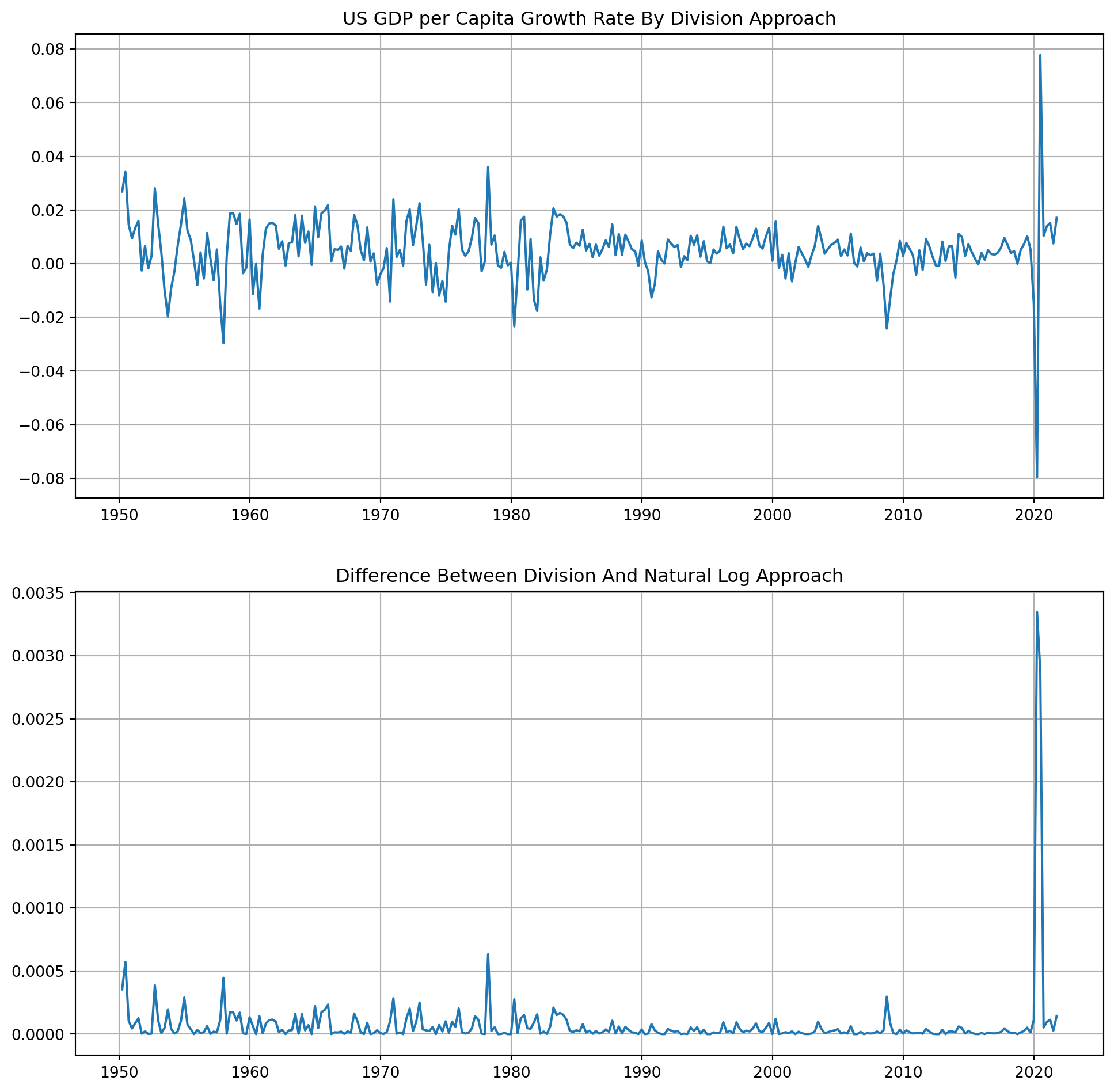
max(df["Gr_rate"])0.07773851590106018max(df["Gr_rate_log_approx"])0.07486487896417238As you can see from log difference growth rate will consistently underestimate the growth rate, however the differences are negligible, mostly difference are under \(5\) basis points, especially post 1980s period, the log difference grow rate approximate real growth rate considerably well. The only exception is the rebound during Covid pandemic, more than \(40\) basis points (\(0.04\%\)).
How Reliable Is The Natural Log Transformation?
We create a series from \(0\) to \(.8\) with step of \(.01\), which means the growth rate ranging from \(0\%\) to \(80 \%\) with step of \(1\%\). The first plot is the comparison of division and natural log approach, as they increase the discrepancy grow bigger too, the second plot is the difference of two approaches, if the growth rate is less than \(20\%\), the error of natural log approach is acceptable.
g = np.arange(0, 0.8, 0.01)
log_g = np.log(1 + g)

fig, ax = plt.subplots(nrows=1, ncols=2, figsize=(16, 8))
ax[0].plot(g, g, label="Division Approach")
ax[0].plot(g, log_g, label="Natural Log Approach")
ax[0].set_xlabel("Real Growth Rate")
ax[0].set_ylabel("Approximated Growth Rate")
ax[0].grid()
ax[0].legend()

ax[1].plot(g, g - log_g, ls="--", lw=3, label="Difference Between Two Approaches")
ax[1].grid()
ax[1].legend()
plt.show()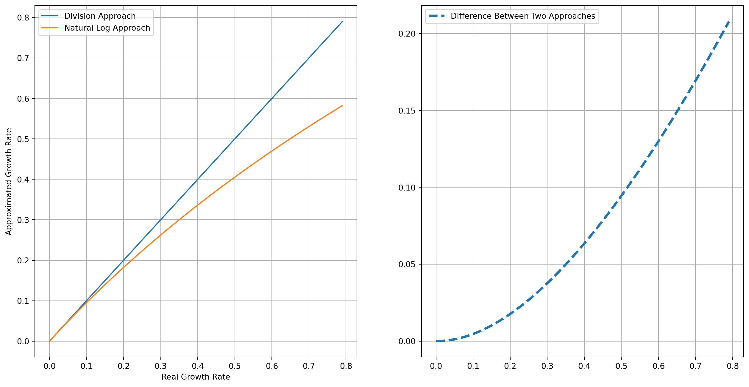
How To Calculate YoY growth rate?
What we have seen above is Quarter on Quarter (QoQ) growth rate, another common way of measuring growth is Year over Year.
If you still using quarterly data, it’s simply \[ g_{YoY, 2021}=\frac{y_{3Q2021}}{y_{3Q2020}}-1 \] where \(y_{3Q2021}\) is the observation on the \(3\)rd quarter of \(2021\), similarly \(y_{3Q2020}\) is from the \(3\)rd quarter of \(2020\).
df["R_GDP_PerCap_tm4"] = df["R_GDP_PerCap"].shift(4)
df = df.dropna()
df| R_GDP_PerCap | R_GDP_PerCap_tm1 | Gr_rate | Gr_rate_log_approx | R_GDP_PerCap_tm4 | |
|---|---|---|---|---|---|
| DATE | |||||
| 1951-04-01 | 17147.0 | 16922.0 | 0.013296 | 0.013209 | 15977.0 |
| 1951-07-01 | 17420.0 | 17147.0 | 0.015921 | 0.015796 | 16524.0 |
| 1951-10-01 | 17375.0 | 17420.0 | -0.002583 | -0.002587 | 16764.0 |
| 1952-01-01 | 17490.0 | 17375.0 | 0.006619 | 0.006597 | 16922.0 |
| 1952-04-01 | 17459.0 | 17490.0 | -0.001772 | -0.001774 | 17147.0 |
| ... | ... | ... | ... | ... | ... |
| 2020-10-01 | 62554.0 | 61915.0 | 0.010321 | 0.010268 | 63360.0 |
| 2021-01-01 | 63428.0 | 62554.0 | 0.013972 | 0.013875 | 62416.0 |
| 2021-04-01 | 64392.0 | 63428.0 | 0.015198 | 0.015084 | 57449.0 |
| 2021-07-01 | 64877.0 | 64392.0 | 0.007532 | 0.007504 | 61915.0 |
| 2021-10-01 | 65986.0 | 64877.0 | 0.017094 | 0.016949 | 62554.0 |
283 rows × 5 columns
df["Gr_rate_log_approx_YoY"] = np.log(df["R_GDP_PerCap"]) - np.log(
    df["R_GDP_PerCap_tm4"]
)
df.head()| R_GDP_PerCap | R_GDP_PerCap_tm1 | Gr_rate | Gr_rate_log_approx | R_GDP_PerCap_tm4 | Gr_rate_log_approx_YoY | |
|---|---|---|---|---|---|---|
| DATE | ||||||
| 1951-04-01 | 17147.0 | 16922.0 | 0.013296 | 0.013209 | 15977.0 | 0.070673 |
| 1951-07-01 | 17420.0 | 17147.0 | 0.015921 | 0.015796 | 16524.0 | 0.052805 |
| 1951-10-01 | 17375.0 | 17420.0 | -0.002583 | -0.002587 | 16764.0 | 0.035799 |
| 1952-01-01 | 17490.0 | 17375.0 | 0.006619 | 0.006597 | 16922.0 | 0.033015 |
| 1952-04-01 | 17459.0 | 17490.0 | -0.001772 | -0.001774 | 17147.0 | 0.018032 |
fig, ax = plt.subplots(figsize=(12, 6))
ax.plot(df["Gr_rate_log_approx_YoY"])
ax.grid()
ax.set_title("US GDP per Capita YoY Growth Rate By Division Approach")
plt.show()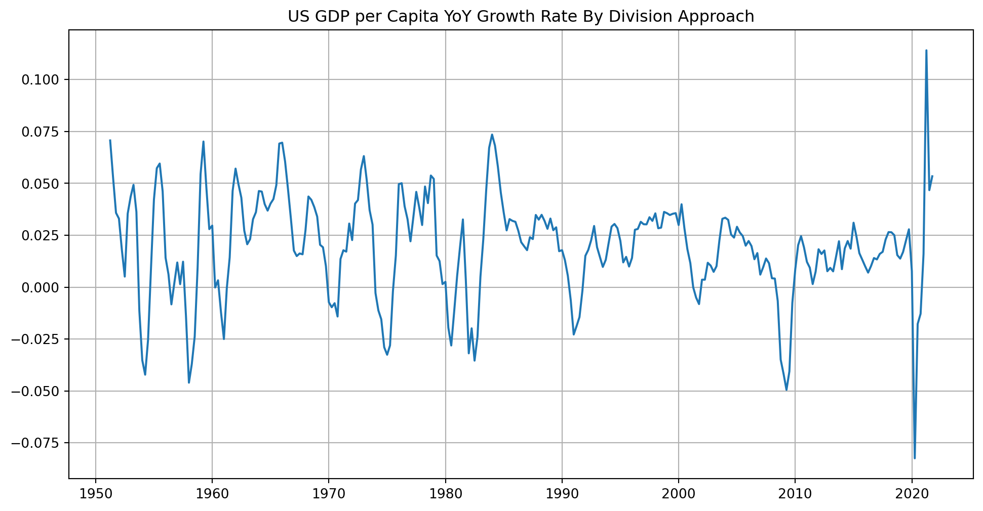
How to Resample Time Series?
By resampling, we can upsample the series, i.e. convert to higher frequency series, or we can downsample the series, i.e. convert to lower frequency series.
For example, you have one series of lower frequency, say annually, but the rest of series are quarterly, in order to incorporate this annual series into the whole dataset, we have to upsample it to quarterly data.
Now we import nominal annual GDP per capita.
start = dt.datetime(1950, 1, 1)
end = dt.datetime(2021, 10, 1)
df = pdr.data.DataReader(["A939RC0A052NBEA"], "fred", start, end)
df.columns = ["Nom_GDP_PerCap_Annual"]
df = df.dropna()
df.head()| Nom_GDP_PerCap_Annual | |
|---|---|
| DATE | |
| 1950-01-01 | 1977.0 |
| 1951-01-01 | 2248.0 |
| 1952-01-01 | 2340.0 |
| 1953-01-01 | 2439.0 |
| 1954-01-01 | 2405.0 |
df_us_Q = df.resample("QS").interpolate(method="linear")  # QS mean quarter start freq
df_us_Q.head()| Nom_GDP_PerCap_Annual | |
|---|---|
| DATE | |
| 1950-01-01 | 1977.00 |
| 1950-04-01 | 2044.75 |
| 1950-07-01 | 2112.50 |
| 1950-10-01 | 2180.25 |
| 1951-01-01 | 2248.00 |
To downsample a series, e.g. to convert daily series into a monthly series
start = dt.datetime(2010, 1, 1)
end = dt.datetime(2021, 10, 1)
df = pdr.data.DataReader(["DEXCHUS"], "fred", start, end)
df.columns = ["USDCNY"]
df = df.dropna()
df.head()| USDCNY | |
|---|---|
| DATE | |
| 2010-01-04 | 6.8273 |
| 2010-01-05 | 6.8258 |
| 2010-01-06 | 6.8272 |
| 2010-01-07 | 6.8280 |
| 2010-01-08 | 6.8274 |
df_M = df.resample("ME").mean()
df_M.head()| USDCNY | |
|---|---|
| DATE | |
| 2010-01-31 | 6.826916 |
| 2010-02-28 | 6.828463 |
| 2010-03-31 | 6.826183 |
| 2010-04-30 | 6.825550 |
| 2010-05-31 | 6.827450 |
fig, ax = plt.subplots(figsize=(15, 8))
ax.plot(df["USDCNY"], label="USDCNY Daily Close")
ax.plot(df_M["USDCNY"], label="USDCNY Monthly Average")
ax.grid()
ax.legend()
plt.show()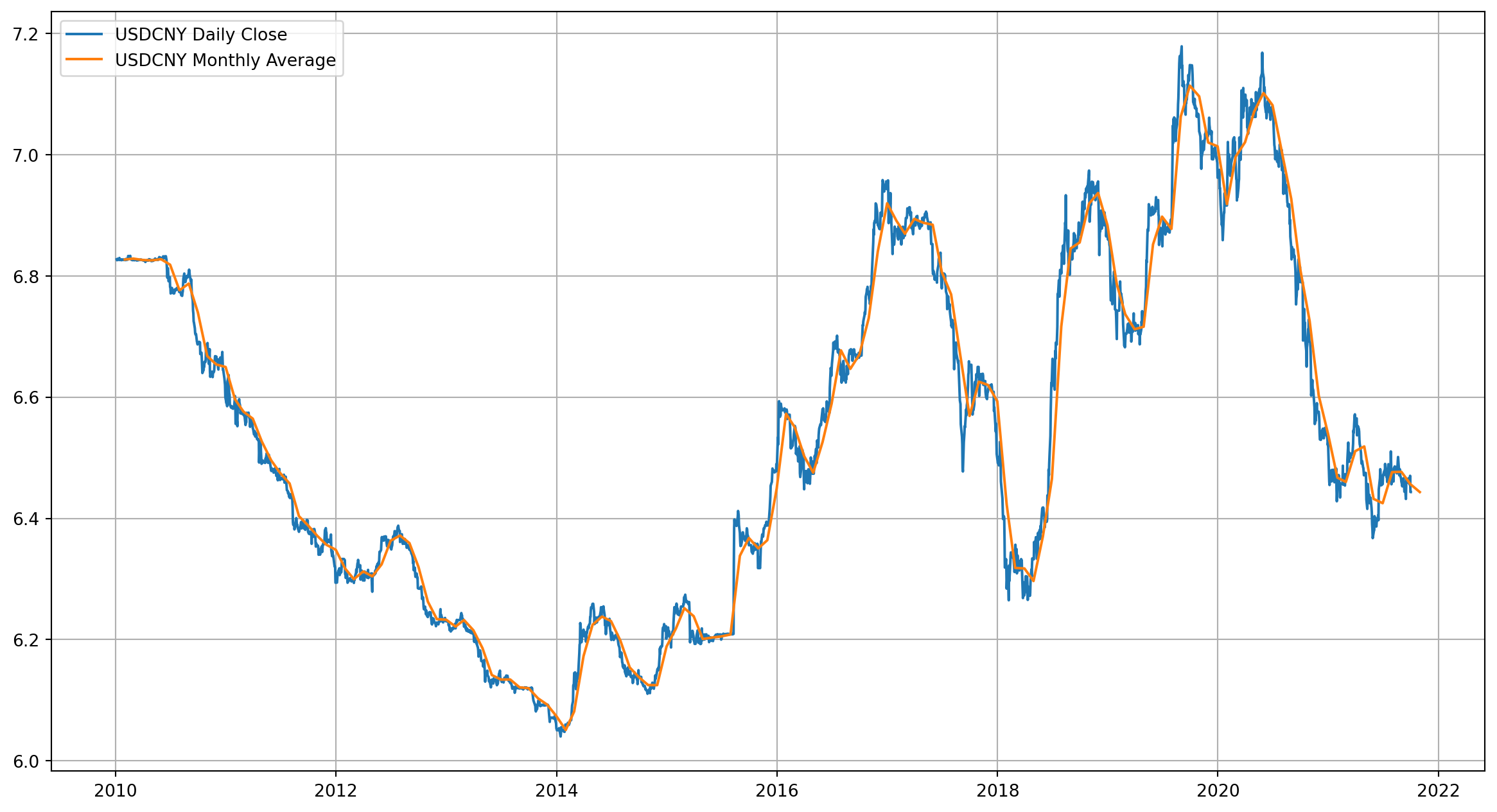
Here’s the full list of frequency supported by Pandas.
B         business day frequency
C         custom business day frequency (experimental)
D         calendar day frequency
W         weekly frequency
M         month end frequency
SM        semi-month end frequency (15th and end of month)
BM        business month end frequency
CBM       custom business month end frequency
MS        month start frequency
SMS       semi-month start frequency (1st and 15th)
BMS       business month start frequency
CBMS      custom business month start frequency
Q         quarter end frequency
BQ        business quarter endfrequency
QS        quarter start frequency
BQS       business quarter start frequency
A         year end frequency
BA, BY    business year end frequency
AS, YS    year start frequency
BAS, BYS  business year start frequency
BH        business hour frequency
H         hourly frequency
T, min    minutely frequency
S         secondly frequency
L, ms     milliseconds
U, us     microseconds
N         nanoseconds
Detrend
The most common tool of detrending in applied macroeconomics is Hodrick-Prescott filter, we assume a time series \(y_t\) can be decomposed into \[ y_t = \tau_t+c_t \] where \(\tau\) is trend and \(c\) is cyclical components.
Trend component minimize objective function over \(\tau\)’s \[ \min _{\tau}\left(\sum_{t=1}^{T}\left(y_{t}-\tau_{t}\right)^{2}+\lambda \sum_{t=2}^{T-1}\left[\left(\tau_{t+1}-\tau_{t}\right)-\left(\tau_{t}-\tau_{t-1}\right)\right]^{2}\right) \]
Academically, \(\lambda\) is suggested to take three distinct values: \[ \begin{align} &\text{Annual}: 6.25 \\ &\text{Quarter}: 1600\\ &\text{Month}: 129600 \end{align} \] However, you can always break these rules, especially in high frequency data.
USDCNY_cycle, USDCNY_trend = hpfilter(np.log(df["USDCNY"]), lamb=10000000)fig, ax = plt.subplots(nrows=2, ncols=1, figsize=(15, 8))
ax[0].plot(np.log(df["USDCNY"]), label="Log USDCNY Daily Close")
ax[0].plot(np.log(df_M["USDCNY"]), label="Log USDCNY Monthly Average")
ax[0].plot(USDCNY_trend, color="red", label="HP-filtered Trend")
ax[0].grid()
ax[0].legend()
ax[1].plot(USDCNY_cycle, label="HP-filtered Cycle")
plt.show()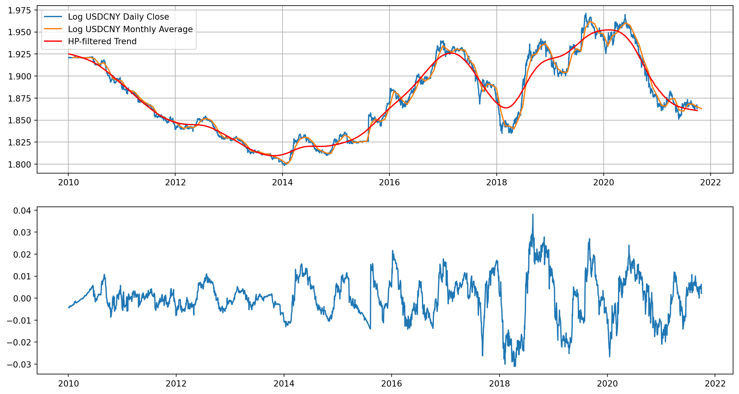
Dynamic Econometric Models
After discussions of autocorrelation, we are officially entering the realm of time series econometrics. For starter, we will discuss dynamic econometric models: distributed-lag model and autogressive model.
In economics and finance, dependent variables and explanatory (independent) variables are rarely instantaneous, i.e. \(Y\) responds to \(X\)’s with a lapse of time.
Distributed-Lag Model (DLM)
Here is a DLM with one explanatory variable \(X\) \[ Y_{t}=\alpha+\beta_{0} X_{t}+\beta_{1} X_{t-1}+\beta_{2} X_{t-2}+\cdots+u_{t} \]
Ad Hoc Estimation Of DLM
If you are estimating variables which have no clear economic relationship or no well-founded theoretical support, go with ad hoc estimation method.
So you start regressing \(X_t\) onto \(Y_t\), then adding \(X_{t-i}\) where \(i \geq 1\) in each round of regression, until \(t\)-statistic starting to be insignificant or signs of coefficients start to be unstable.
\[\begin{align} \hat{Y}_t &= a + b_0X_t\\ \hat{Y}_t &= a + b_0X_t+b_1X_{t-1}\\ \hat{Y}_t &= a + b_0X_t+b_1X_{t-1}+b_2X_{t-2}\\ \hat{Y}_t &= a + b_0X_t+b_1X_{t-1}+b_1X_{t-1}+b_3X_{t-3}\\ \end{align}\]
But be aware that ad hoc method is bring significant problem of multicollinearity.
Koyck Approach To DLM
Koyck approach assumes that all \(\beta\)’s are of the same sign, furthermore \[ \beta_{k}=\beta_{0} \lambda^{k} \quad k=0,1, \ldots \] where \(\lambda\) is the rate of decay, \(0<\lambda<1\).
lamda = np.linspace(0.3, 0.9, 6)
beta_0 = 1
k = np.linspace(0, 4)
fig, ax = plt.subplots(figsize=(12, 8))
for i in lamda:
    beta_k = beta_0 * i**k
    ax.plot(k, beta_k, label=r"$\lambda$ = %.2f" % i)
ax.legend()
ax.axhline(y=0.5, zorder=-10, color="k")
plt.show()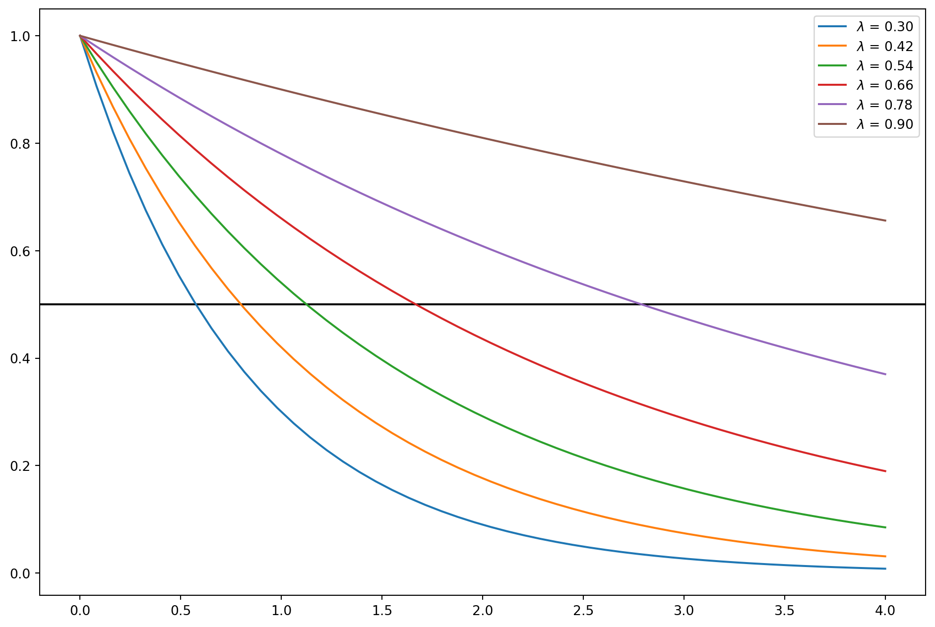
There are three perks of Koyck approach:
- By assuming nonnegative values for \(λ\), \(\beta\)’s sign are stable;
- by assuming \(λ < 1\), lesser weight is given to the distant \(β\)’s than the current ones;
- The sum of the \(β\)’s, which gives the long-run multiplier, is finite, i.e. \[ \sum_{k=0}^{\infty} \beta_{k}=\beta_{0}\left(\frac{1}{1-\lambda}\right) \]
Naturally, the infinite distributed lag model can be rewritten as \[ Y_{t}=\alpha+\beta_{0} X_{t}+\beta_{0} \lambda X_{t-1}+\beta_{0} \lambda^{2} X_{t-2}+\cdots+u_{t} \]
Lag both sides one period \[ Y_{t-1}=\alpha+\beta_{0} X_{t-1}+\beta_{0} \lambda X_{t-2}+\beta_{0} \lambda^{2} X_{t-3}+\cdots+u_{t-1} \]
Multiply by \(\lambda\) \[ \lambda Y_{t-1}=\lambda \alpha+\lambda \beta_{0} X_{t-1}+\beta_{0} \lambda^{2} X_{t-2}+\beta_{0} \lambda^{3} X_{t-3}+\cdots+\lambda u_{t-1} \] Join with original equation \[ Y_{t}-\lambda Y_{t-1}=\alpha(1-\lambda)+\beta_{0} X_{t}+\left(u_{t}-\lambda u_{t-1}\right) \]
Rearrange, we obtain \[ Y_{t}=\alpha(1-\lambda)+\beta_{0} X_{t}+\lambda Y_{t-1}+v_{t} \] where \(v_t = (u_t − λu_{t−1})\).
This is called Koyck transformation which simplifies original infinite DLM into an \(AR(1)\).
An Example Of Consumption And Income
We import macro data from FRED, \(PCE\) is real personal consumption expenditure and \(DI\) is real disposable income per capita.
start = dt.datetime(2002, 1, 1)
end = dt.datetime(2021, 10, 1)
df_exp = pdr.data.DataReader(["PCEC96", "A229RX0"], "fred", start, end)
df_exp.columns = ["PCE", "DI"]
df_exp = df_exp.dropna()
df_exp.head()| PCE | DI | |
|---|---|---|
| DATE | ||
| 2007-01-01 | 11181.0 | 39803.0 |
| 2007-02-01 | 11178.2 | 39906.0 |
| 2007-03-01 | 11190.7 | 40007.0 |
| 2007-04-01 | 11201.5 | 40037.0 |
| 2007-05-01 | 11218.0 | 40029.0 |
Define a function for lagging, which is handy in \(R\)-style formula.
def lag(x, n):
    if n == 0:
        return x
    if isinstance(x, pd.Series):
        return x.shift(n)
    else:
        x = pd.Series(x)
        return x.shift(n)
    x = x.copy()
    x[n:] = x[0:-n]
    x[:n] = np.nan
    return x
The model is \[ PCE_t = \alpha(1-\lambda) + \beta_0 DI_t + \lambda PCE_{t-1}+ v_t \]
DLM = smf.ols(formula="PCE ~ 1 + lag(DI, 0) + lag(PCE, 1)", data=df_exp)
DLM_results = DLM.fit()
print(DLM_results.summary())
OLS Regression Results
==============================================================================
Dep. Variable: PCE R-squared: 0.978
Model: OLS Adj. R-squared: 0.977
Method: Least Squares F-statistic: 3819.
Date: Sun, 27 Oct 2024 Prob (F-statistic): 1.80e-144
Time: 17:33:38 Log-Likelihood: -1156.9
No. Observations: 177 AIC: 2320.
Df Residuals: 174 BIC: 2329.
Df Model: 2
Covariance Type: nonrobust
===============================================================================
coef std err t P>|t| [0.025 0.975]
-------------------------------------------------------------------------------
Intercept -127.5084 150.359 -0.848 0.398 -424.270 169.253
lag(DI, 0) 0.0216 0.007 3.132 0.002 0.008 0.035
lag(PCE, 1) 0.9365 0.023 40.059 0.000 0.890 0.983
==============================================================================
Omnibus: 253.714 Durbin-Watson: 1.669
Prob(Omnibus): 0.000 Jarque-Bera (JB): 29238.841
Skew: -5.950 Prob(JB): 0.00
Kurtosis: 64.830 Cond. No. 5.39e+05
==============================================================================
Notes:
[1] Standard Errors assume that the covariance matrix of the errors is correctly specified.
[2] The condition number is large, 5.39e+05. This might indicate that there are
strong multicollinearity or other numerical problems.The estimated results:
beta_0 = DLM_results.params[1]
lamda = DLM_results.params[2]
alpha = DLM_results.params[0] / (1 - DLM_results.params[2])

print("beta_0 = {}".format(beta_0))
print("lambda = {}".format(lamda))
print("alpha = {}".format(alpha))
beta_0 = 0.021625743412386718
lambda = 0.9364710981601484
alpha = -2007.0925201650587/tmp/ipykernel_2699/3362829195.py:1: FutureWarning:
Series.__getitem__ treating keys as positions is deprecated. In a future version, integer keys will always be treated as labels (consistent with DataFrame behavior). To access a value by position, use `ser.iloc[pos]`
/tmp/ipykernel_2699/3362829195.py:2: FutureWarning:
Series.__getitem__ treating keys as positions is deprecated. In a future version, integer keys will always be treated as labels (consistent with DataFrame behavior). To access a value by position, use `ser.iloc[pos]`
/tmp/ipykernel_2699/3362829195.py:3: FutureWarning:
Series.__getitem__ treating keys as positions is deprecated. In a future version, integer keys will always be treated as labels (consistent with DataFrame behavior). To access a value by position, use `ser.iloc[pos]`
Any \(\beta_k\) is given by \(\beta_{k}=\beta_{0} \lambda^{k}\)
def beta_k(lamda, k, beta_0):
    return beta_0 * lamda**k
beta_k(lamda, 1, beta_0)0.020251883681927384The long run multiplier given by \(\sum_{k=0}^{\infty} \beta_{k}=\beta_{0}\left(\frac{1}{1-\lambda}\right)\)
beta_0 * (1 / (1 - lamda))0.3404079526969081 / (1 - lamda)15.740867086304664Median lag, the lags that it takes to decay the first half. From our example, that \(PCE\) adjusts to \(DI\) with substantial lag, around \(9\) month to have half impact.
-np.log(2) / np.log(lamda)10.560373002569747Mean lag
lamda / (1 - lamda)14.740867086304664Stochastic Processes
Unstrictly speaking, stochastic processes is a subject of mathematics that studies a family of random variables which are indexed by time. Since time series data is a series of realization of a stochastic process, before investigating further, we will introduce some basic concepts of stochastic processes.
For instance, we denote \(GDP\) as \(Y_t\) which is a stochastic process, therefore \(Y_1\) and \(Y_2\) are two different random variables, if \(Y_1 = 12345\), then it is a realization of \(t_1\). You can think of stochastic process as population and realization as sample as in cross-sectional data.
Stationary Stochastic Processes
A stochastic process is said to be stationary if its mean and variance are constant over time and the value of the covariance between the two time periods depends only on the distance \(k\) between the two time periods and not the actual time at which the covariance is computed. Mathematically, a weak stationary process should satisfy three conditions:
\[\begin{align} Mean:& \quad E\left(Y_{t}\right)=\mu\\ Variance:&\quad E\left(Y_{t}-\mu\right)^{2}=\sigma^{2}\\ Covariance:&\quad E\left[\left(Y_{t}-\mu\right)\left(Y_{t+k}-\mu\right)\right] = \gamma_{k} \end{align}\]
Most of time weak stationary process will suffice, rarely we require a process to be strong stationary which means all moments are time-invariant. A common feature of time-invariant time series is mean reversion.
Why do we care about stationarity?
If a time series is nonstationary, we can only study the behavior in a particular episode and the outcomes can’t be generalized to other episodes. Therefore forecasting nonstationary time series would absolutely be of little value.
Nonstationary Stochastic Processes
The most common type of nonstationary process is random walk, and two subtypes are demonstrated below: with/without drift.
Random Walk With Drift
A random walk without drift can be modeled with a \(AR(1)\) where \(\rho=1\) and constant term is \(0\) \[ Y_t = Y_{t-1}+u_t \] The mean and variance can be shown \[\begin{align} E\left(Y_{t}\right)&=E\left(Y_{0}+\sum u_{t}\right)=Y_{0}\\ \operatorname{Var}\left(Y_{t}\right)&=t \sigma^{2} \end{align}\] There are lots of financial time series resemble random walk process, for example, we will generate a random walk with the same length of \(EURUSD\), let’s see if you can visually differentiate them
start = dt.datetime(2000, 1, 1)
end = dt.datetime(2021, 10, 1)
df_eurusd = pdr.data.DataReader(["DEXUSEU"], "fred", start, end)
df_eurusd.columns = ["EURUSD"]
df_eurusd = df_eurusd.dropna()
def rw_wdr(init_val, length):
rw_array = []
rw_array.append(init_val)
last = init_val
for i in range(length):
current = last + np.random.randn() / 100
rw_array.append(current)
last = current
return rw_arrayrw = rw_wdr(1.0155, len(df.index) - 1)
df_rw = pd.DataFrame(rw, index=df.index, columns=["Simulated Asset Price"])
fig, ax = plt.subplots(figsize=(16, 8))
ax.plot(df_rw, color="#2c90b8", label="Random Walk Without Drift")
ax.plot(df_eurusd, color="tomato", label="EURUSD")
ax.grid()
ax.legend(fontsize=16)
plt.show()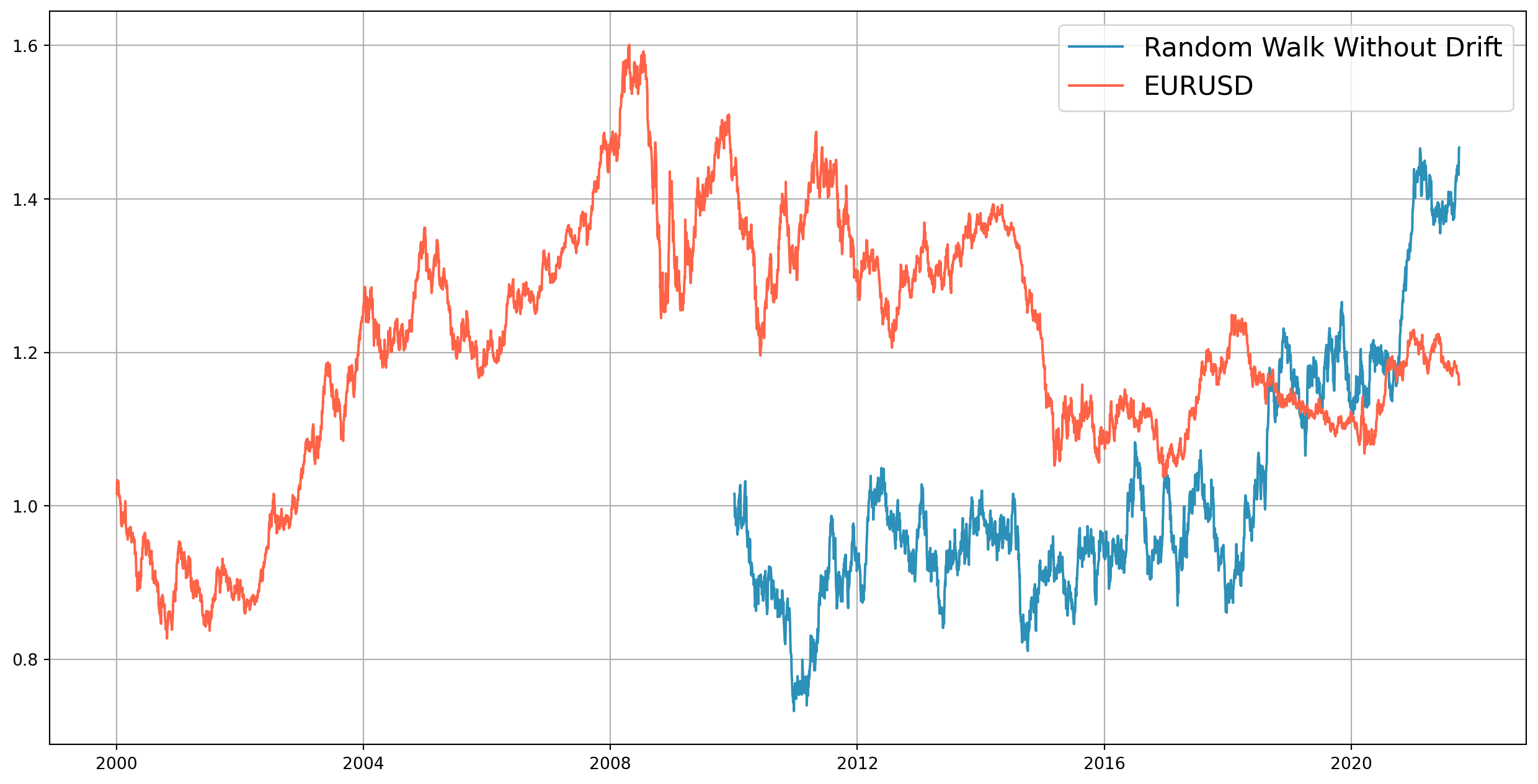
First order difference of random walk is stationary.
fig, ax = plt.subplots(figsize=(16, 8))
ax.plot(
    df_rw.diff().dropna(),
    color="#2c90b8",
    label="Random Walk Without Drift First Order Diff",
    lw=0.2,
)
ax.grid()
ax.legend(fontsize=16)
plt.show()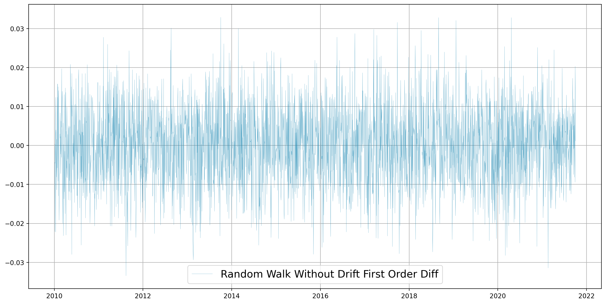
Note that if we rewrite the model \[ \Delta Y_{t}=\left(Y_{t}-Y_{t-1}\right)=u_{t} \] it becomes stationary, hence it is difference stationary process (DSP).
Random Walk With Drift
Random walk with drift can be modeled by \[ Y_{t}=\delta+Y_{t-1}+u_{t} \] And mean and variance are \[ \begin{aligned} E\left(Y_{t}\right) &=Y_{0}+t \cdot \delta \\ \operatorname{Var}\left(Y_{t}\right) &=t \sigma^{2} \end{aligned} \]
def rw_dr(dr_param, init_val, length):
    rw_array = []
    rw_array.append(init_val)

    last = init_val
    for i in range(length):
        current = dr_param + last + 50 * np.random.randn()
        rw_array.append(current)
        last = current
    return rw_array
rw = rw_dr(5, 1, len(df.index) - 1)df_rw = pd.DataFrame(rw, index=df.index, columns=["Simulated Asset Price"])
fig, ax = plt.subplots(nrows=2, ncols=1, figsize=(16, 14))
ax[0].plot(df_rw, color="#2c90b8", label="Random Walk With Drift")
ax[1].plot(
df_rw.diff().dropna(),
color="#2c90b8",
label="Random Walk With Drift First Order Diff",
lw=0.2,
)
ax[0].grid()
ax[0].legend(fontsize=16)
ax[1].legend()
plt.show()
As long as \(\rho=1\), we call it unit root problem, thus the terms nonstationarity, random walk, unit root, and stochastic trend can be treated synonymously.
If we rewrite the model \[ \left(Y_{t}-Y_{t-1}\right)=\Delta Y_{t}=\beta_{1}+u_{t} \]
which is also a DSP, however if \(\beta\neq 0\), the first difference exhibits a positive or negative trend, which is called stochastic trend.
Trend Stationary Process
Consider the model \[ Y_{t}=\beta_{1}+\beta_{2} t+u_{t} \] If we subtract \(E(Y_t)\) from \(Y_t\), resulting series will be stationary, hence it is trend stationary process (TSP). Deterministic trend with \(AR(1)\) component \[ Y_{t}=\beta_{1}+\beta_{2} t+\beta_{3} Y_{t-1}+u_{t} \]
Integrated Stochastic Processes
Any time series, after a first order difference, becomes stationary, we call it integrated of order 1 denoted \(Y_t\sim I(1)\). If a time series has to be differenced twice to be stationary, we call such time series integrated of order 2 denoted \(Y_t\sim I(2)\).
Most of economic and financial time series are \(I(1)\).
Properties of Integrated Series
- If \(X_{t} \sim I(0)\) and \(Y_{t} \sim I(1)\), then \(Z_{t}=\left(X_{t}+Y_{t}\right)=I(1)\)
- If \(X_{t} \sim I(d)\), then \(Z_{t}=\left(a+b X_{t}\right)=I(d)\), where \(a\) and \(b\) are constants. Thus, if \(X_{t} \sim I(0)\), then \(Z_{t}=\) \(\left(a+b X_{t}\right) \sim I(0)\)
- If \(X_{t} \sim I\left(d_{1}\right)\) and \(Y_{t} \sim I\left(d_{2}\right)\), then \(Z_{t}=\left(a X_{t}+b Y_{t}\right) \sim I\left(d_{2}\right)\), where \(d_{1}<d_{2}\)
- If \(X_{t} \sim I(d)\) and \(Y_{t} \sim I(d)\), then \(Z_{t}=\left(a X_{t}+b Y_{t}\right) \sim I\left(d^{*}\right) ; d^{*}\) is generally equal to \(d\), but in some cases \(d^{*}<d\)
Spurious Regression
The best way to understand spurious regression is to generate two random walk series then regression one onto the other. Let’s simulate two assets’ price \(Y_t\) and \(X_t\)
\[\begin{aligned} Y_{t} &= \alpha_1+\alpha_2 Y_{t-1}+u_{t} \\ X_{t} &=\beta_1+\beta_2 X_{t-1}+v_{t} \end{aligned}\]def rw_dr(dr_param, slope_param, init_val, length):
rw_array = []
rw_array.append(init_val)
last = init_val
for i in range(length):
current = dr_param + slope_param * last + 50 * np.random.randn()
rw_array.append(current)
last = current
return rw_array
N = 5000
X = rw_dr(2, 1, 0, N)
Y = rw_dr(0, 1, 0, N)
dates = pd.date_range("19900101", periods=N + 1)
df = pd.DataFrame([X, Y]).T
df.columns = ["Asset_X", "Asset_Y"]
df.index = dates
df.plot(figsize=(12, 8), grid=True)
plt.show()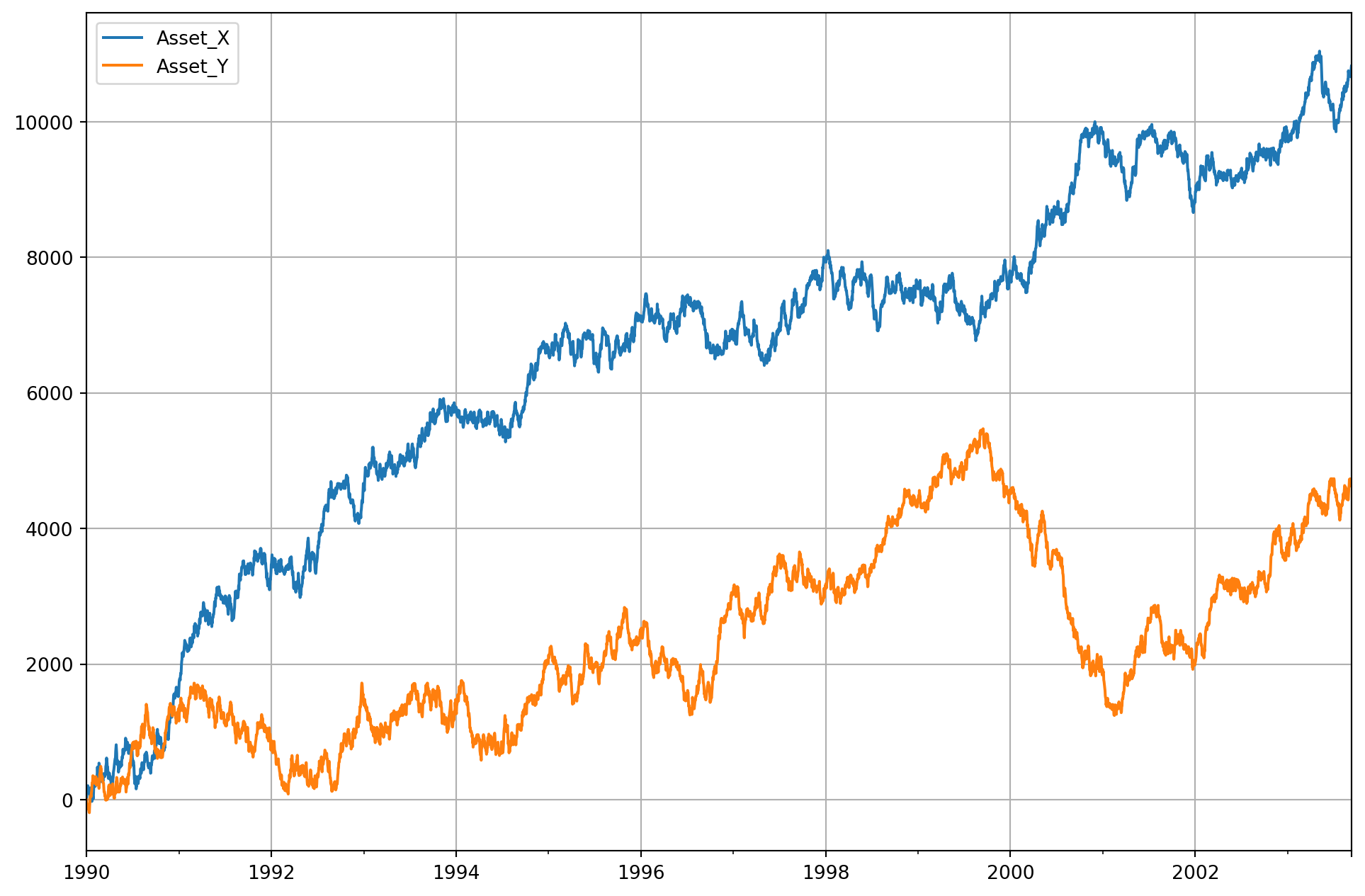
model = smf.ols(formula="Asset_Y ~ Asset_X", data=df)
results = model.fit()
print(results.summary())
OLS Regression Results
==============================================================================
Dep. Variable: Asset_Y R-squared: 0.465
Model: OLS Adj. R-squared: 0.464
Method: Least Squares F-statistic: 4338.
Date: Sun, 27 Oct 2024 Prob (F-statistic): 0.00
Time: 17:33:40 Log-Likelihood: -41610.
No. Observations: 5001 AIC: 8.322e+04
Df Residuals: 4999 BIC: 8.324e+04
Df Model: 1
Covariance Type: nonrobust
==============================================================================
coef std err t P>|t| [0.025 0.975]
------------------------------------------------------------------------------
Intercept 28.4886 37.731 0.755 0.450 -45.480 102.457
Asset_X 0.3548 0.005 65.861 0.000 0.344 0.365
==============================================================================
Omnibus: 279.794 Durbin-Watson: 0.003
Prob(Omnibus): 0.000 Jarque-Bera (JB): 327.845
Skew: 0.625 Prob(JB): 6.45e-72
Kurtosis: 3.110 Cond. No. 1.88e+04
==============================================================================
Notes:
[1] Standard Errors assume that the covariance matrix of the errors is correctly specified.
[2] The condition number is large, 1.88e+04. This might indicate that there are
strong multicollinearity or other numerical problems.Note that \(t\)-statistic of \(X\) is highly significant, and \(R^2\) is relatively low though \(F\)-statistic extremely significant. You will see different results when running codes on your computer, because I didn’t set random seeds in Python.
We know the data generating processes of \(X\) and \(Y\) are absolutely irrelevant, but regression results say otherwise. This a phenomenon of spurious regression. You can see the \(dw\) is almost \(0\), which signals strong autocorrelation issue.
An \(R^2 > dw\) is a good rule of thumb to suspect that the estimated regression is spurious. Also note that all statistic tests are invalid because \(t\)-statistics are not distributed as \(t\)-distribution.
Tests Of Stationarity
Autocorrelation Function And Correlogram
Autocorrelation function (ACF) at lag \(k\) is defined as \[\begin{aligned} \rho_{k} &=\frac{\gamma_{k}}{\gamma_{0}}=\frac{\text { covariance at lag } k}{\text { variance }} \end{aligned}\] In practice, we can only compute sample autocorrelation function, \(\hat{\rho}_k\) \[\begin{aligned} &\hat{\gamma}_{k}=\frac{\sum\left(Y_{t}-\bar{Y}\right)\left(Y_{t+k}-\bar{Y}\right)}{n-k} \\ &\hat{\gamma}_{0}=\frac{\sum\left(Y_{t}-\bar{Y}\right)^{2}}{n-1} \end{aligned}\]Note that \(\hat{\rho}_0 = 1\).
If we plot \(\hat{\rho}\) against \(k\), we obtain correlogram, here is a correlogram of a white noise
from statsmodels.graphics import tsaplots

X = np.random.randn(1000)
plot_acf(X, lags=100, color="red").set_size_inches(16, 6)
plt.show()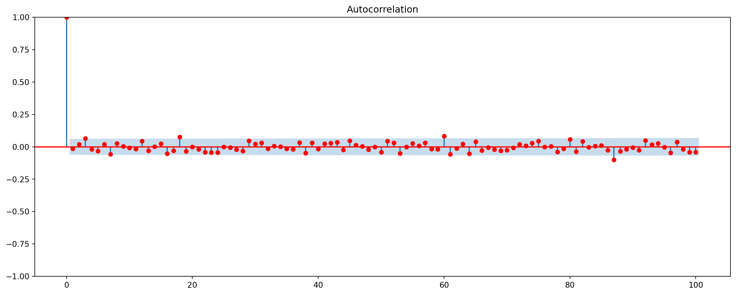
plt.figure(figsize=(16, 6))
pd.plotting.autocorrelation_plot(X).set_xlim([0, 100])
plt.show()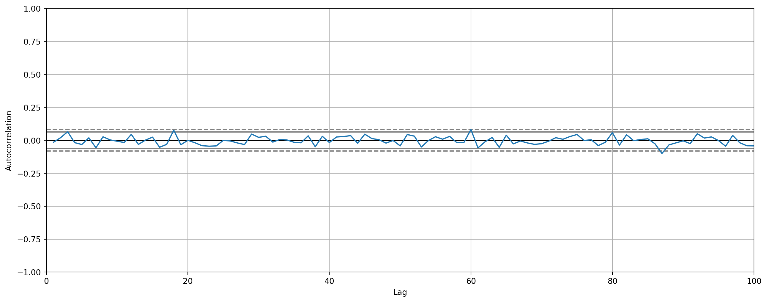
Obviously, autocorrelation at various lags hover around \(0\), which is a sign of stationarity.
Here is the correlogram of monthly urban consumers’ CPI in US. Note the old tradition in econometrics is to computer ACF up to \(1/3\) length of time series, we are following this rule below.
df = pdr.data.DataReader(["CPIAUCSL"], "fred", start, end)
df.columns = ["CPI_Urban"]

plt.figure(figsize=(16, 6))
pd.plotting.autocorrelation_plot(df["CPI_Urban"]).set_xlim([0, np.round(len(df) / 3)])
plt.show()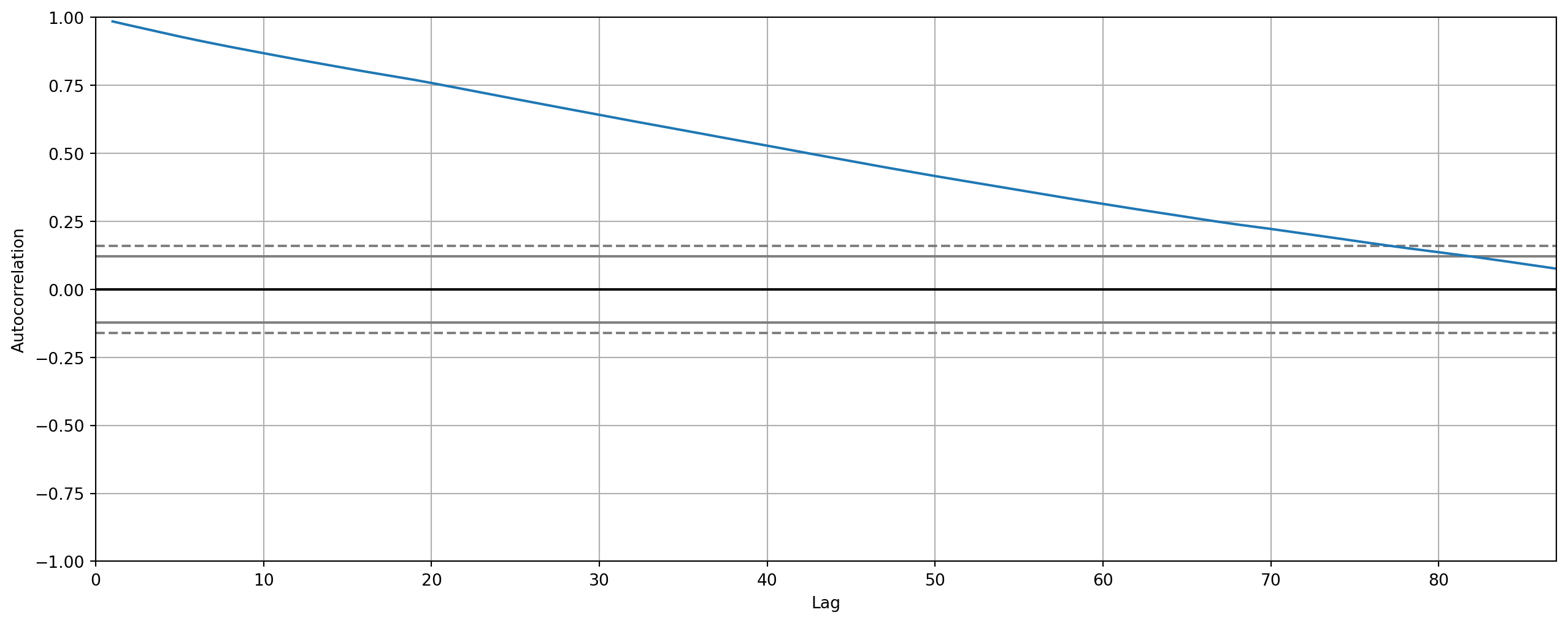
Ljung-Box Test
Apart from the Breusch-Godfrey and Durbin-Watson test that we have discussed in the chapter of autocorrelation, we will introduce one more common autocorrelation test in time series, Ljung-Box Test (LB test). \[ \mathrm{LB}=n(n+2) \sum_{k=1}^{m}\left(\frac{\hat{\rho}_{k}^{2}}{n-k}\right) \sim \chi^{2}_m \]
The hypotheses are \[ H_0: \text{No autocorrelation presents}\\ H_1: \text{Autocorrelation presents for specified lags} \]
There are many controversial debates about when and how to use these statistics, but those academic debates belong to academia, we go lightly here. LB test is group test which depends on any specification of lags. If you want to check if first \(10\) lags if it shows any sign of autocorrelation, we use the code as below
sm.stats.acorr_ljungbox(df["CPI_Urban"], lags=[10], return_df=True, boxpierce=True)| lb_stat | lb_pvalue | bp_stat | bp_pvalue | |
|---|---|---|---|---|
| 10 | 2308.449335 | 0.0 | 2244.617168 | 0.0 |
The test shows overwhelmingly evidence for autocorrelation up to lag \(10\). Note that we also add boxpierce argument in the function, this is a variant of LB test, usually printed for reference.
Dickey–Fuller (DF) test
If we suspect that \(Y_t\) follows a unit root process, why don’t we simply regress \(Y_t\) onto \(Y_{t-1}\), i.e. \[ Y_{t}=\rho Y_{t-1}+u_{t} \quad-1 \leq \rho \leq 1 \] The problem is that if \(\rho=1\), the \(t\)-statistic is severely biased, let’s simulate the process and examine if this is the case.
However, some manipulation can circumvent the issue \[\begin{aligned} Y_{t}-Y_{t-1} &=\rho Y_{t-1}-Y_{t-1}+u_{t} \\ &=(\rho-1) Y_{t-1}+u_{t}\\ \Delta Y_t &= \delta Y_{t-1}+u_{t} \end{aligned}\]where \(\delta = \rho-1\). If \(\delta =0\), i.e. \(\rho=1\), then \(\Delta Y_t = u_t\), therefore \(Y_t\) is unstationary; if \(\delta <0\), then \(\rho <1\), in that case \(y_t\) is stationary.
The last equation \(\Delta Y_t = \delta Y_{t-1}+u_{t}\) is the one to estimate and hypotheses are \[ H_0: \delta = 0, \text{unstationary}\\ H_1: \delta < 0, \text{stationary} \]
It turns out the \(t\)-statistic calculated on \(\delta\) doesn’t really follow a \(t\)-distribution, it actually follows \(\tau\)-distribution or Dickey-Fuller distribution, therefore we call it Dickey-Fuller test.
from statsmodels.tsa.stattools import adfullerresults_dickeyfuller = adfuller(X)
print("ADF Statistic: %f" % results_dickeyfuller[0])
print("p-value: %f" % results_dickeyfuller[1])ADF Statistic: -16.890158
p-value: 0.000000Transforming Nonstationary Time Series
In academia, unfortunately transformation of nonstationarity is still a controversial topic. Jame Hamilton argues that we should never use HP filter due to its heavy-layered differencing, i.e. the cyclical components of HP-filtered series are the fourth difference of its corresponding trend component.
Also because most of economic and financial time series exhibit features of random walk, the cyclical components are merely artifacts of applying the filter.
However, let’s not be perplexed by sophisticated academic discussion. Here’s the rule of thumb.
HP filter or F.O.D.?
If you want to do business cycle analysis with structural macro model, use HP-filter.
If you want to do ordinary time series modeling, use first order difference.
Cointegration
We have seen the invalid estimated results from regression of nonstationary time series onto another nonstationary time series, which possibly would cause a spurious regression.
However, if both series share a common trend, the regression between them will not be necessarily spurious.
start = dt.datetime(1980, 1, 1)
end = dt.datetime(2021, 10, 1)
df = pdr.data.DataReader(["PCEC96", "A229RX0"], "fred", start, end).dropna()
df.columns = ["real_PCE", "real_DPI"]
df.head()| real_PCE | real_DPI | |
|---|---|---|
| DATE | ||
| 2007-01-01 | 11181.0 | 39803.0 |
| 2007-02-01 | 11178.2 | 39906.0 |
| 2007-03-01 | 11190.7 | 40007.0 |
| 2007-04-01 | 11201.5 | 40037.0 |
| 2007-05-01 | 11218.0 | 40029.0 |
model = smf.ols(formula="np.log(real_PCE) ~ np.log(real_DPI)", data=df)
results = model.fit()print(results.summary()) OLS Regression Results
==============================================================================
Dep. Variable: np.log(real_PCE) R-squared: 0.801
Model: OLS Adj. R-squared: 0.800
Method: Least Squares F-statistic: 707.5
Date: Sun, 27 Oct 2024 Prob (F-statistic): 1.47e-63
Time: 17:33:42 Log-Likelihood: 322.82
No. Observations: 178 AIC: -641.6
Df Residuals: 176 BIC: -635.3
Df Model: 1
Covariance Type: nonrobust
====================================================================================
coef std err t P>|t| [0.025 0.975]
------------------------------------------------------------------------------------
Intercept -0.8891 0.388 -2.293 0.023 -1.654 -0.124
np.log(real_DPI) 0.9662 0.036 26.598 0.000 0.895 1.038
==============================================================================
Omnibus: 128.807 Durbin-Watson: 0.595
Prob(Omnibus): 0.000 Jarque-Bera (JB): 1484.516
Skew: -2.558 Prob(JB): 0.00
Kurtosis: 16.190 Cond. No. 1.40e+03
==============================================================================
Notes:
[1] Standard Errors assume that the covariance matrix of the errors is correctly specified.
[2] The condition number is large, 1.4e+03. This might indicate that there are
strong multicollinearity or other numerical problems.dickey_fuller = adfuller(results.resid)
print("ADF Statistic: %f" % dickey_fuller[0])
print("p-value: %f" % dickey_fuller[1])ADF Statistic: -2.594071
p-value: 0.094229Note that we are able to reject null hypothesis of nonstationarity with \(5\%\) siginificance level.
plot_acf(results.resid, lags=100, color="red").set_size_inches(16, 6)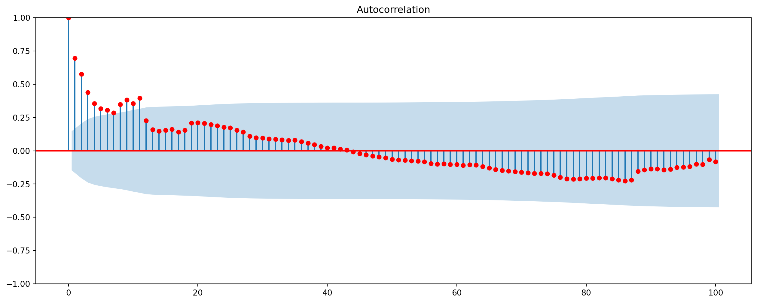
The disturbance terms can be seen as a linear combination of \(PCE\) and #DPI# \[ u_{t}=\ln{PCE}_{t}-\beta_{1}-\beta_{2} \ln{DPI}_{t} \] If both variables are \(I(1)\), but residuals are \(I(0)\), we say that the two variables are cointegrated, the regression is also known as cointegrating regression. Economically speaking, two variables will be cointegrated if they have a long-term, or equilibrium, relationship between them.
One of the key considerations prior to testing for cointegration, is whether there is theoretical support for the cointegrating relationship. It is important to remember that cointegration occurs when separate time series share an underlying stochastic trend. The idea of a shared trend should be supported by economic theory.
One thing to note here, in cointegration context, we usually perform a Engle–Granger (EG) or augmented Engle–Granger (AEG) test, they are essential DF test,
\[ H_0: \text{No cointegration}\\ H_1: \text{Cointegreation presents} \]
from statsmodels.tsa.stattools import coint

coint_test1 = coint(df["real_PCE"], df["real_DPI"], trend="c", autolag="BIC")
coint_test2 = coint(df["real_PCE"], df["real_DPI"], trend="ct", autolag="BIC")
def coint_output(res):
output = pd.Series(
[res[0], res[1], res[2][0], res[2][1], res[2][2]],
index=[
"Test Statistic",
"p-value",
"Critical Value (1%)",
"Critical Value (5%)",
"Critical Value (10%)",
],
)
print(output)Without linear trend.
coint_output(coint_test1)Test Statistic -2.700932
p-value 0.199244
Critical Value (1%) -3.959385
Critical Value (5%) -3.370868
Critical Value (10%) -3.068498
dtype: float64With linear trend.
coint_output(coint_test2)Test Statistic -4.624758
p-value 0.003608
Critical Value (1%) -4.415983
Critical Value (5%) -3.834688
Critical Value (10%) -3.536555
dtype: float64Error Correction Mechanism
Error Correction Mechanism (ECM) is an phenomenon that any variable deviates from its equilibrium will correct its own error gradually.
\[ u_{t-1}=\ln{PCE}_{t-1}-\beta_{1}-\beta_{2} \ln{DPI}_{t-1} \] \[ \Delta \ln{PCE}_{t}=\alpha_{0}+\alpha_{1} \Delta \ln{DPI}_{t}+\alpha_{2} \mathrm{u}_{t-1}+\varepsilon_{t} \]
Suppose \(u_{t-1}> 0\) and \(\Delta DPI_t =0\), it means \(PCE_t\) is higher than equilibrium. In order to correct this temporary error, \(\alpha_2\) has to be negative to adjust back to the equilibrium, hence \(\Delta \ln{PCE_t}<0\).
We can get \(u_{t-1}\) by \(\hat{u}_{t-1}\) \[ \hat{u}_{t-1}=\ln{PCE}_{t-1}-\hat{\beta}_{1}-\hat{\beta}_{2} \ln{DPI}_{t-1} \]
df_new = {
    "Delta_ln_PCE": df["real_PCE"].diff(1),
    "Delta_ln_DPI": df["real_DPI"].diff(1),
    "u_tm1": results.resid.shift(-1),
}
df_new = pd.DataFrame(df_new).dropna()
df_new| Delta_ln_PCE | Delta_ln_DPI | u_tm1 | |
|---|---|---|---|
| DATE | |||
| 2007-02-01 | -2.8 | 103.0 | -0.026827 |
| 2007-03-01 | 12.5 | 101.0 | -0.026587 |
| 2007-04-01 | 10.8 | 30.0 | -0.024922 |
| 2007-05-01 | 16.5 | -8.0 | -0.023549 |
| 2007-06-01 | 0.5 | -55.0 | -0.020731 |
| ... | ... | ... | ... |
| 2021-05-01 | -42.7 | -1514.0 | 0.034722 |
| 2021-06-01 | 137.9 | -250.0 | 0.026396 |
| 2021-07-01 | -35.2 | 312.0 | 0.034967 |
| 2021-08-01 | 91.9 | -126.0 | 0.048574 |
| 2021-09-01 | 34.4 | -589.0 | 0.055237 |
176 rows × 3 columns
model_ecm = smf.ols(formula="Delta_ln_PCE ~ Delta_ln_DPI + u_tm1", data=df_new)
results_ecm = model_ecm.fit()
print(results_ecm.summary())
OLS Regression Results
==============================================================================
Dep. Variable: Delta_ln_PCE R-squared: 0.124
Model: OLS Adj. R-squared: 0.114
Method: Least Squares F-statistic: 12.24
Date: Sun, 27 Oct 2024 Prob (F-statistic): 1.06e-05
Time: 17:33:42 Log-Likelihood: -1144.0
No. Observations: 176 AIC: 2294.
Df Residuals: 173 BIC: 2303.
Df Model: 2
Covariance Type: nonrobust
================================================================================
coef std err t P>|t| [0.025 0.975]
--------------------------------------------------------------------------------
Intercept 21.9591 12.246 1.793 0.075 -2.211 46.129
Delta_ln_DPI -0.0135 0.009 -1.551 0.123 -0.031 0.004
u_tm1 1445.4546 309.016 4.678 0.000 835.527 2055.382
==============================================================================
Omnibus: 73.636 Durbin-Watson: 1.725
Prob(Omnibus): 0.000 Jarque-Bera (JB): 6805.275
Skew: 0.263 Prob(JB): 0.00
Kurtosis: 33.458 Cond. No. 3.56e+04
==============================================================================
Notes:
[1] Standard Errors assume that the covariance matrix of the errors is correctly specified.
[2] The condition number is large, 3.56e+04. This might indicate that there are
strong multicollinearity or other numerical problems.